Pivot Tables are the most powerful tools that you can use in your Google Sheets. A slicer is the feature that can filter out Pivot Tables easily. Very useful when you need to keep all your data together but you want to present parts of it (slices)
In a previous example you can see how to create a simple Pivot Table in Google Sheets. We used an Education case study where the teacher Amanda wanted to have a summary of their students grades ready for the Teacher-Parent conference. Amanda keeps track of the grades in a simple Google Sheet like this
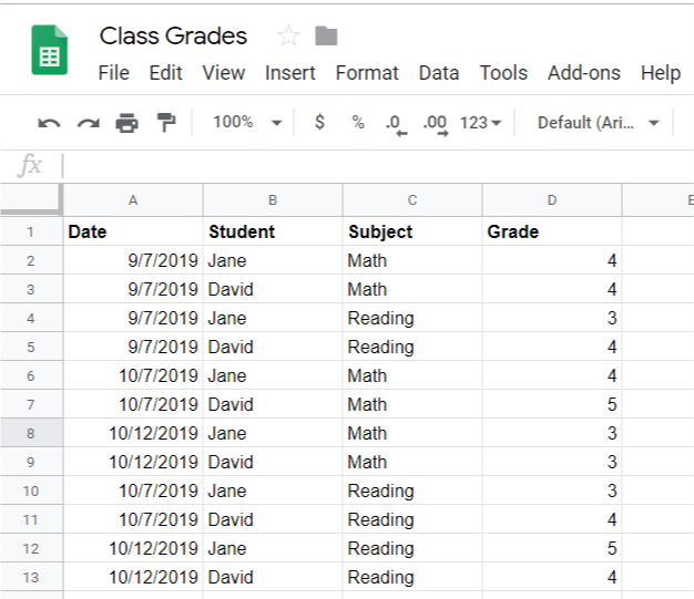
Amanda prepared in the previous example a summary like this using a simple Google Sheets Pivot Table

Case Study
In the following example, we’ll continue with the same dataset and pivot table we already created and prepare a more advanced summary. Amanda’s School Principle is asking for an average of grades in her class without the student’s names and he also wants it broken down by subject. On top of that, he wants to be able to select each student easily and see how he or she performed throughout the year.
Adding a slicer to Google Sheets
In the rows, add the Subject field and remove the Row
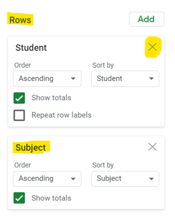
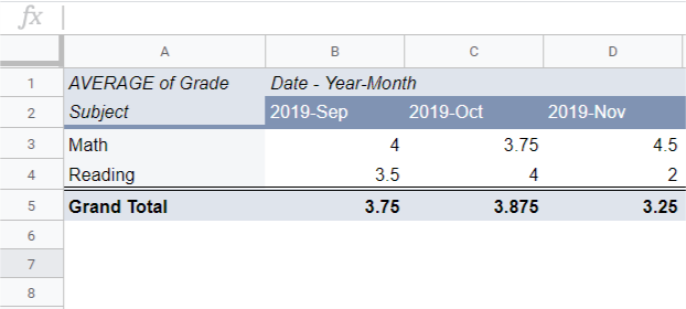
Now your pivot table looks like this. It will contain the grade average by subject for the entire year and no student name.
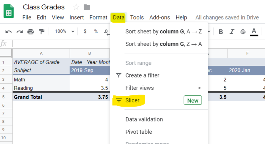
In order to create a Student selection we will insert a slicer from Data – Slicer. Make sure your Pivot Table is selected.
What is a Slicer in Google Sheets
A slicer is nothing more than a filter that one can use to quickly filter out a pivot table. The first thing you have to do is to select the column that you want to use for the slicer. Choose Student in the Slicer Section.
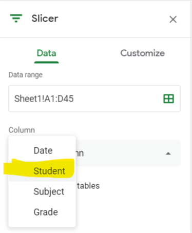
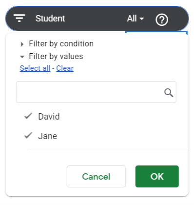
The resulting slicer is a dropdown that allows you to choose a student name and to show only the data for that student in the Pivot Table. Great feature to use if you want to focus on one Student only but still have all the data summarized for the entire class with a click of a button
That is all. If you found this helpful, share with your colleagues.
