How to use VLOOKUP in Excel

Excel Vlookup is the most powerful formula in Excel. Also vlookup is one of the formulas that are least used because so many users are scared of it. In this tutorial you will learn:

how to use vlookup in Excel
what is the vlookup syntax
how to do a vlookup between two spreadsheets
why is my vlookup not working
why is xlookup coming and how will it improve vlookup

If you know vlookup and pivot tables you will find the most value out of Excel.

We’ll continue with our example of the Grocery Store that keeps track of the sales of fruits and vegetables for every day of the year.

This dataset contains the sales by day of every type of product they have in store. To keep it simple, we only have 4 products: apples, oranges, cucumbers and broccoli

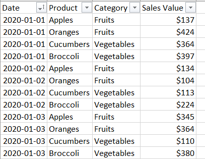
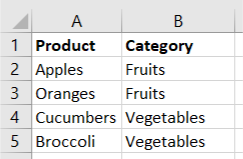
As you notice, these 4 products are actually grouped in 2 categories: fruits and vegetables. Whoever is typing in this data has to make sure they type the correct category, or the summary will not be accurate.

To have vlookup help with this task, create a category worksheet looking like this

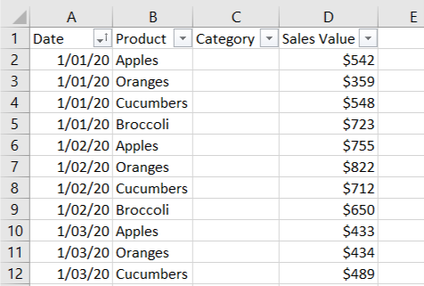
Once you have that, remove all records in the Category column in the main data-set

What is the vlookup syntax

Let’s learn the syntax of this function to know how to use better. A good guide on syntax can be found in Excel if you click on the fx button in the formula bar. This will display a windows with each of the functions elements and the result of the function. See the example for the vlookup function

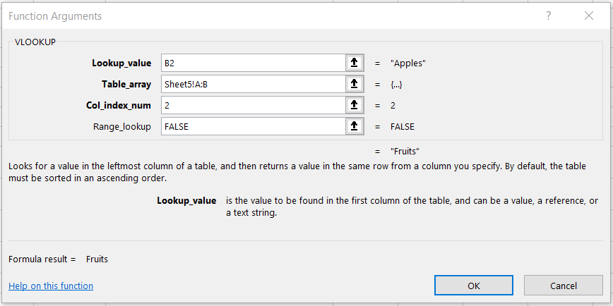
But, with this in mind, let’s backtrack and start writing the formula in the formula bar. Click in the cell C2 and enter the following: =vlookup(

Once you type that, excel will help you filling in the rest of the formula.

Let’s now break down the 4 elements of the vlookup formula. Vookup is looking for a lookup_value into a table. So we have to tell it what to look for, where to look, where in the table will it find it and if it should match it exactly.

lookup_value – this is the value that you look for. In this case, you would look for “apples” that can be found in B2. Type B2 and then comma

table_array -this is where you tell the formula where to find the category for this lookup_value. In other words, where is the information that the apples belong to the category fruits. While still editing the formula, click on the worksheet that holds the category information above and select columns A and B (first column that contains the products and ending with the last column that contains the category). Type again comma after that.

You can now see the partial formula in the formula bar and the guide for what the formula should be. So you can see that the table_array is now setup as range A:B in Sheet5.

Once you type comma, the formula moves to the next field

col_index_num – this is the column index number where you would find the information you lookup. You know your product information is in column A (index 1) and the category is in the next column (index 2). So type 2. You’ll find the category information in column with the index 2 (second column). This is obvious with a small dataset but if you have a large dataset with many columns you have to count the columns starting from 1 and type in the number of the column where the lookup information is.

The last field is range_lookup. This is the field that tells the formula to look for an exact match (FALSE) or an approximate match (TRUE). Most of the time this value will be FALSE.

Once you type the last part of the formula, close the bracket and hit Enter.

=vlookup(B2,Sheet5!A:B,2,FALSE)

How does vlookup actually work

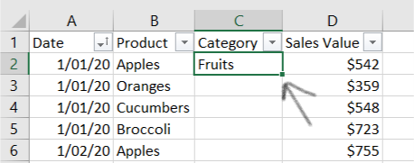
The formula will go look for “Apples” in the “Category” table and bring the information from the second column once it matches exactly the word “apple”. It will find “Apples” in the cell A2 and will go in the second column and retrieve the value “Fruits” and bring it back to the first table.

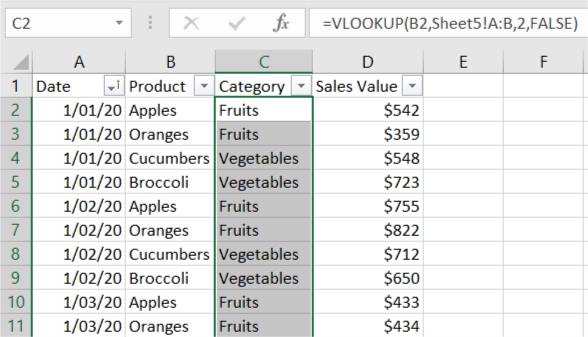
While selecting the cell C2, double click on the little square on the bottom right to copy down the formula all the way to the bottom

And there it is. You used vlookup to fill up the category column with the correct category information.

Here’s another simple example that demonstrates how data should be organized for VLOOKUP to work.

How to do a vlookup between two spreadsheets

In the example above, we had the list of categories in the same file, just in a different tab. But many times in real life the value that you need to find is in a different file. You may have a list of categories that is maintained by a different department. You can choose to copy the list to your file but then, you have to keep track of categories modifications and removal and always keep your list up to date and sync with the other department.

The best way to do this is to do the vlookup in the other worksheet.

The process is very similar. Let’s use the same example as above but move the list of categories into a new file called category.xlsx

The first step is to open both files.

The easiest way to do this is to click on the fx Function Arguments window and to see the function in the visual window. Place your cursor in the “Table_array” cell and delete the contents of that cell (if you had the table array from the same file)

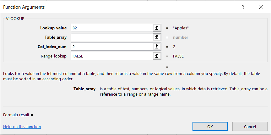
While your cursor is in the Table_array cell, you are in formula editing mode. Go to the other open file with Alt-Tab or selecting it from the taskbar and select the columns where the table array is

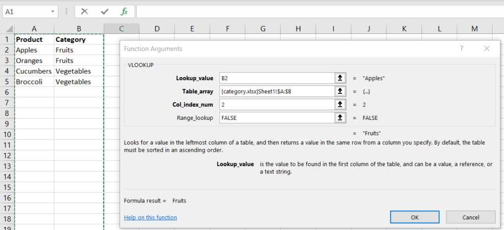
click OK to finish the formula.

Click on the formula now and you’ll see the full path of the file and the table array location once you close the other file.

But what happens if this file moves?

Let’s try it.

Nothing will happen while the file with vlookup is still open. The formulas and values will still display. But if you close the file and open it again, the following message appears

Excel detected a broken link. To fix it, click on “Edit Links”

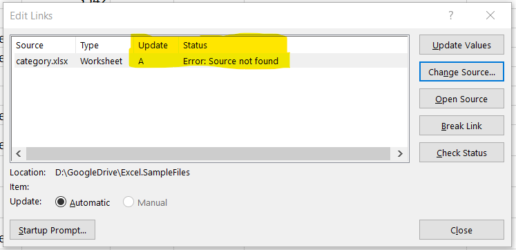
You can now use “Update Values” to point to the new location of the file or even Change Source to point to a similar file that has the same data.

Why is my vlookup not working

In the last section of this comprehensive vlookup tutorial we’ll address the most common causes of why vlookup will stop working or error out.

Data mismatch

If your data is not matching 100% vlookup will error out. For example, if you look for the word Apples and the category list has it listed as apple you get the following error

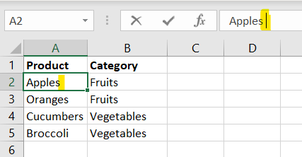
It can be tricky when there is a space in the wrong place for example (both in the source or destination word. In the example below, there is a space after Apples. you can only see it if you place the cursor in the edit mode in the formula bar.

Relative vs Absolute Table array reference

Another tricky one is when you use relative versus absolute reference to specify a table array. In the example above I used the entire columns A:B as table array. That means that if I add any new categories in the A:B columns, the formulas will continue to pick them up.

But what if I specify exactly where the categories are. Like this

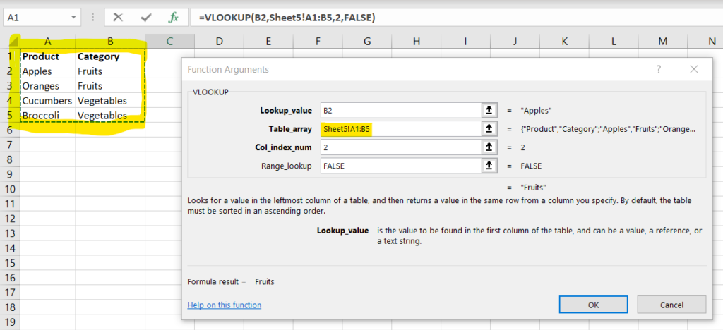
It will work out. For the first cell. But once we copy the formula down, this happens

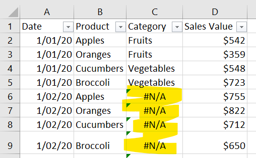
The reason for that is that the formula will take our relative reference to the range A1:B5 and tun it into A2:B6, A3:B7 etc. Once you reach the 6th column, the table array is completely outside the range

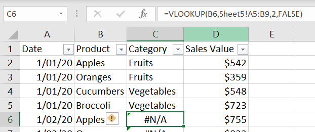
If you want to use exact references to the range, use absolute reference by adding the $ sign for the first and last cell of the range.

=VLOOKUP(B2,Sheet5!$A$1:$B$5,2,FALSE)

The lookup range can’t be found in the leftmost column of the range

This is one of the vlookup limitations that will be fixed by the release of xlookup in 2019. The lookup range has to be in the first column of the table array. If you have this range

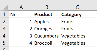
and you have to look for the values in column B (Product) your table array has to be specified as B:C and not as A:C. vlookup will search for the lookup value in the first column. If you specify A:C, column A does not have any products and you’ll get an error

Column Index number is out of range

This can happen a lot if you look for a value into a large range and you have to count the columns to get tot the results column. You may be off by one and either get the worn result or get a #REF error

In the example below, I look for the value in the third column (3) in a two column range (B:C)

These are the main reasons vlookup fails. If you find others, leave us a comment. We can add them in the list.

Why is xlookup coming and how will it improve vlookup

Vlookup was a trusted formula for generations. But it had some limitations. Xlookup is coming to take care of those limitations. For more details on xlookup see the post about the advantages of xlookup.

If this was helpful, share with your colleagues.