SUMIF formula is great for summarizing data in a large dataset. A better method to summarize the data is a pivot table. But if only a quick summary is required, SUMIF might be an easier method.
Here is the dataset
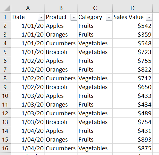
In a previous tutorial you can see how to do a pivot table of this 1464 row dataset and sum up all the sales by category and products.
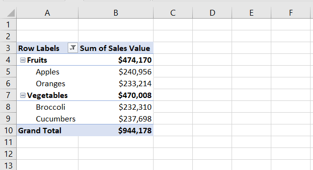
The SUMIF method
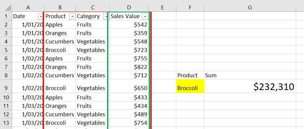
Another way to obtain the same result as in the pivot table is to use a SUMIF function. For example, the SUMIF could summarize the sales for Broccoli into a quick formula like this.
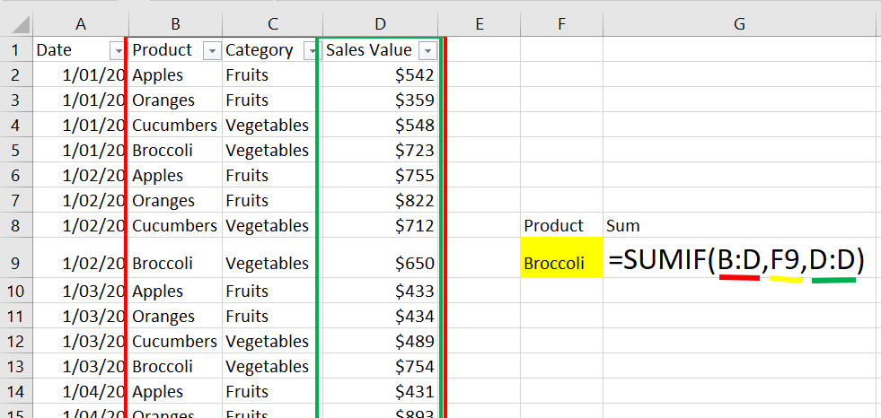
The SUMIF formula is looking in the B:D range (marked in red) for the criteria in F9 (marked in yellow) and is summarizing all the values in the sum_range D column (marked in green). In other words, it is looking in the list of sales for the product Broccoli and it is adding all the sales values in the column D. Click on the fx button on the formula bar to see the details of the function.
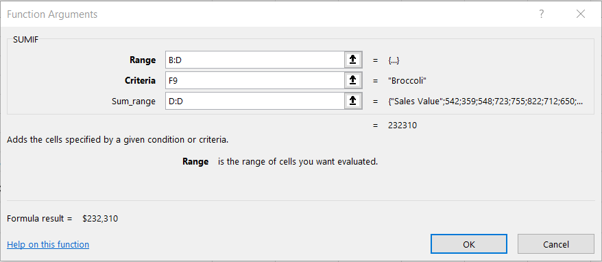
And here is the result of the formula. Notice it is the same as the result in the pivot table above.
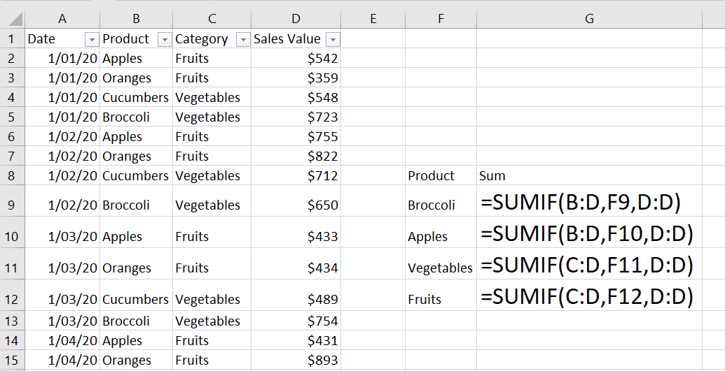
Let’s look at more SUMIF variations. Notice when SUMIF is done on the values in the category column, the range where the lookup is done is reduced to the columns C and D. That is because the Range has to start in the column where the values to be looked up are in.
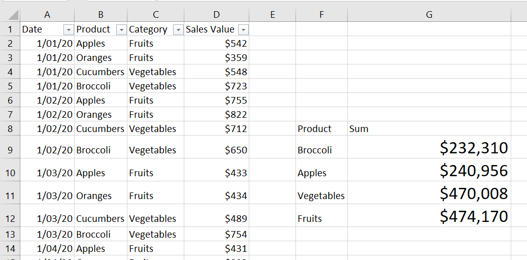
And here are the results of these formulas
SUMIF and COUNTIF are good formulas for summarizing large sets of data. As mentioned before, pivot tables can do the same thing for all the products and categories. If only a few summaries are required, use SUMIF and COUNTIF.
