If in the previous example we studied how to create a simple pivot table from a simple data-set, in this example we add an additional column to categorize our products in order to create a Multi-Level Row Pivot Table
Case Study
A grocery store wants to keep track of daily sales of the main fruits thei are selling: Apples and Oranges. They start with a blank Excel sheet and each day add two lines. One for the sales of Apples and one for the sales of Oranges. Towards the end of the month, the store manager wants to summarize the sales on Apples and Oranges for the month.
In the example below, the store ads more products and introduces a Category. The store manager wants to summarize the sales by Product but in the same time by Category
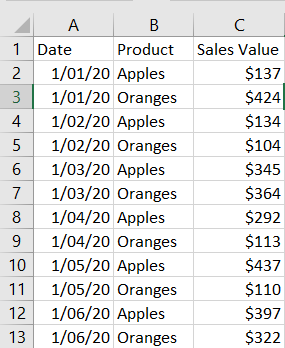
Initial Data-set
The store was selling only Fruits so the daily sales were listed by Product only
New Data-Set
In this example, we are adding cucumbers and broccoli on top of the apples and oranges. We are creating two categories for these products. The categories are Fruits and Vegetables and they will be listed in a new column called “Category”.
You can Save these categories in a separate sheet and use vlookup to pull the information in this worksheet.
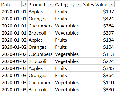
We now have a total of 124 records for 1 month and we want to know not just the total sales per product but also per category.
Insert a new Pivot Table
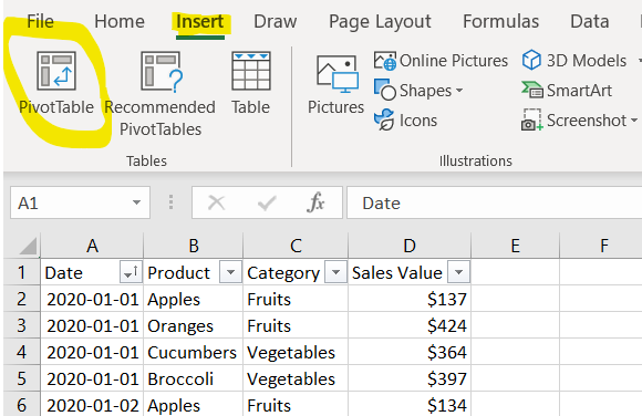
Similar to the previous example, we will click on a cell in the Data-set and click on Insert – Pivot Table.
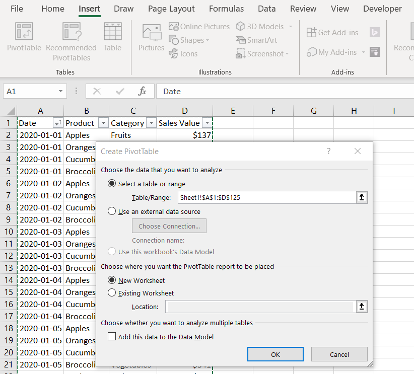
Excel will again Detect the Data-Set boundaries and suggest to place the pivot table in a new worksheet.
We can now drag and drop the Pivot Table Fields as below in the boxes below or select them using the select box in the following order.
First select Sales Value. Excel will detect it contains values and place it in the Values Category. Since Excel detected a different number in each cell it assumes that you want to sum it up. (You can change that later)
Next, select Category. Now Excel will create a Summary by Category.
And last, select Product. Now Excel will break down the Category into the specific Products.
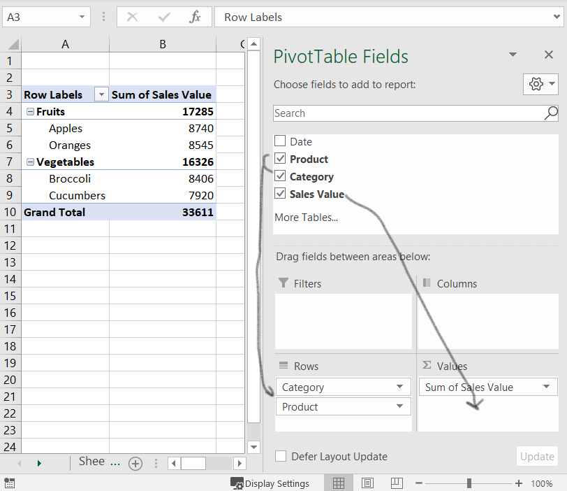
Now you have a summary by Category and Products of the Sales of one month.
You can add more levels in the Rows section if you have more data. You may have the sales person, the Store Location in case you have more locations. Keep adding these rows in the Rows section on top to categorize the sales even more.
But what happens if we want to see how these sales are doing from Month to Month?
See the next Post to see a Multi-Level Row and Multi Level Column Pivot Table.
If this was helpful, you can help this website by sharing this tutorial.
