Here are a few methods to get a day name (Monday, Tuesday, Wednesday etc) from a date field in Excel. If you prefer video, see the tutorials below.
Use Excel TEXT formula
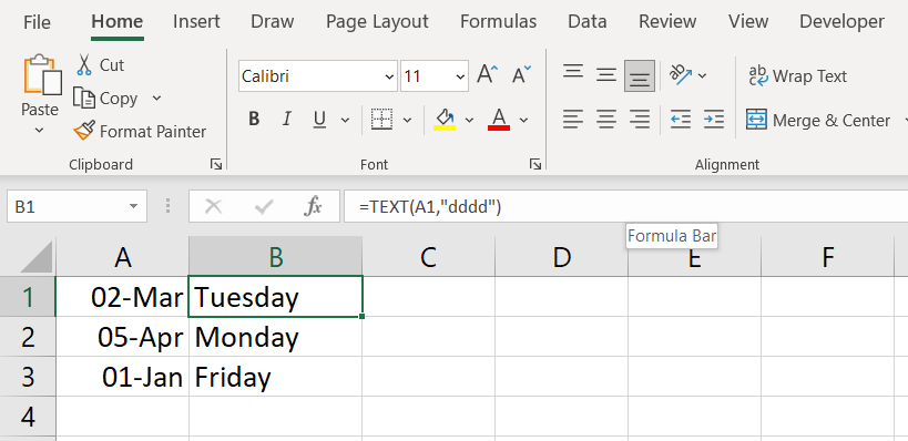
The Excel Text formula will extract the day in a specified text type format. Here is how it works.
The formula for this is =TEXT(cell,”dddd”)
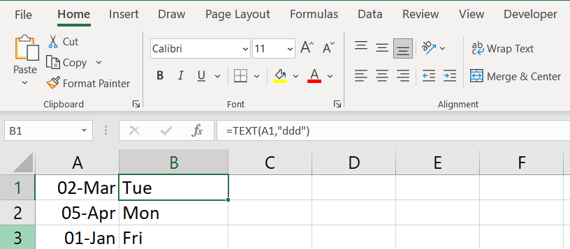
Short Day Name for Date
An alternative text for this is a short name for the day (Mon, Tue, Wed, etc). To achieve that, use the formula =TEXT(cell,”ddd”)
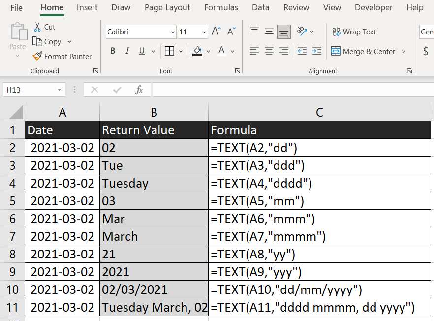
Day Month and Year Names for Date
The TEXT function can be used for pulling name of other components of the date. For example, you can use it to extract the Month or the Year. Here are a few examples
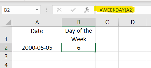
Use the WEEKDAY formula to get the day number
Use WEEKDAY formula if you want the day number in the week. (Day 1, Day 2 etc). This formula also gives you the flexibility to define the start of your week as preferred (Day 1 is Monday, Day one is Sunday etc)
The formula is =WEEKDAY(cell, [return_type])
By default, WEEKDAY returns 1 for Sunday and 7 for Saturday.
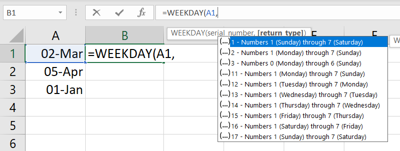
Define the Start of the Week
The optional parameter is [return_type] and it lets you make your choice for the start of the week.
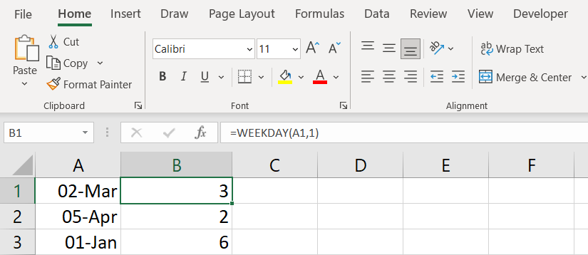
The result of this function is this
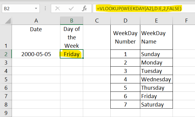
Convert the day number to a Day Name using VLOOKUP
When using WEEKDAY() formula you get a number (the day number if the week). If you want to the name of the day (Monday, Tuesday etc) then you need to perform an additional operation. We need to do a VLOOKUP on the number in order to find the corresponding day.
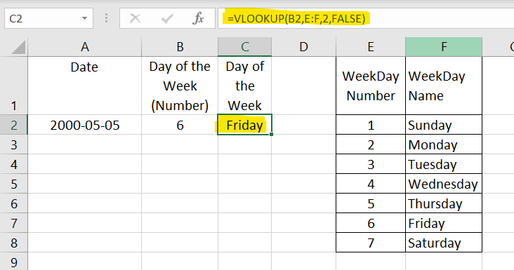
For that to work, we need a reference table like this
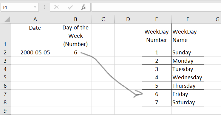
So we need to pull up the corresponding day name from the table for the number 6. To do that we will write a VLOOKUP function to lookup for the value in B2 in the E:F range
=VLOOKUP(B2,E:F,2,FALSE)
Combining formulas
In order to save space and reduce the number of elements on the page, it might be useful sometimes to combine formulas. The two formulas we used to get the Day of the week were:
in Cell B2 =WEEKDAY(A2)
in Cell C2 =VLOOKUP(B2,E:F,2,FALSE)
Notice that the second formula is using the result of the first formula saved in B2. So we can combine the two formulas like this
in Cell C2 =VLOOKUP(WEEKDAY(A2),E:F,2,FALSE)
Writing it like this we replaced the B2 in the second formula with the actual formula we used to get the value in B2. This would help us eliminate a step and cleaning up the worksheet from unnecessary items