Slicers in Excel are filters that help slice the data in a modern and dynamic way. Before slicers, filters were the only way to “slice” a pivot table data. The slicers were a step forward to a dashboard and a first step to Power BI.
If you are a Google Sheets user, you can use slicers there too. See here how to use slicers in Google Sheets.
How to filter a pivot table without slicers
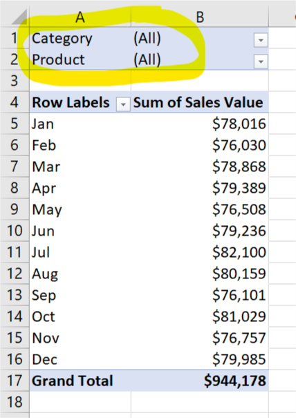
Before slicers, filters were the only way to filter the data. The problem with using filters is that the filters are independent. The data below has two categories (Fruits and Vegetables) and two fruits in the fruits category (Apples and Oranges) as well as two vegetables in the vegetables category (Broccoli and Cucumbers)

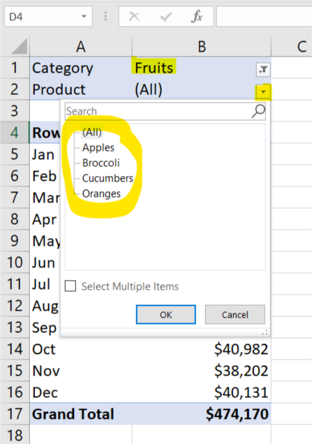
So if you choose Apples in the Category Filter, you still have all the options in the second category.

If you would choose the wrong Product that does not belong in the Fruits Category, the pivot table will show no data.

Filtering a pivot table with slicers.
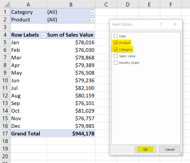
A better method to filter a pivot table is a slicer. To add slicers, go to the Insert tab on the ribbon and click on Slicer. Make sure the pivot table is selected by clicking anywhere on the pivot table.

Select the fields you want to add as Slicers. in this example, we’ll add Category and Product as Slicers.

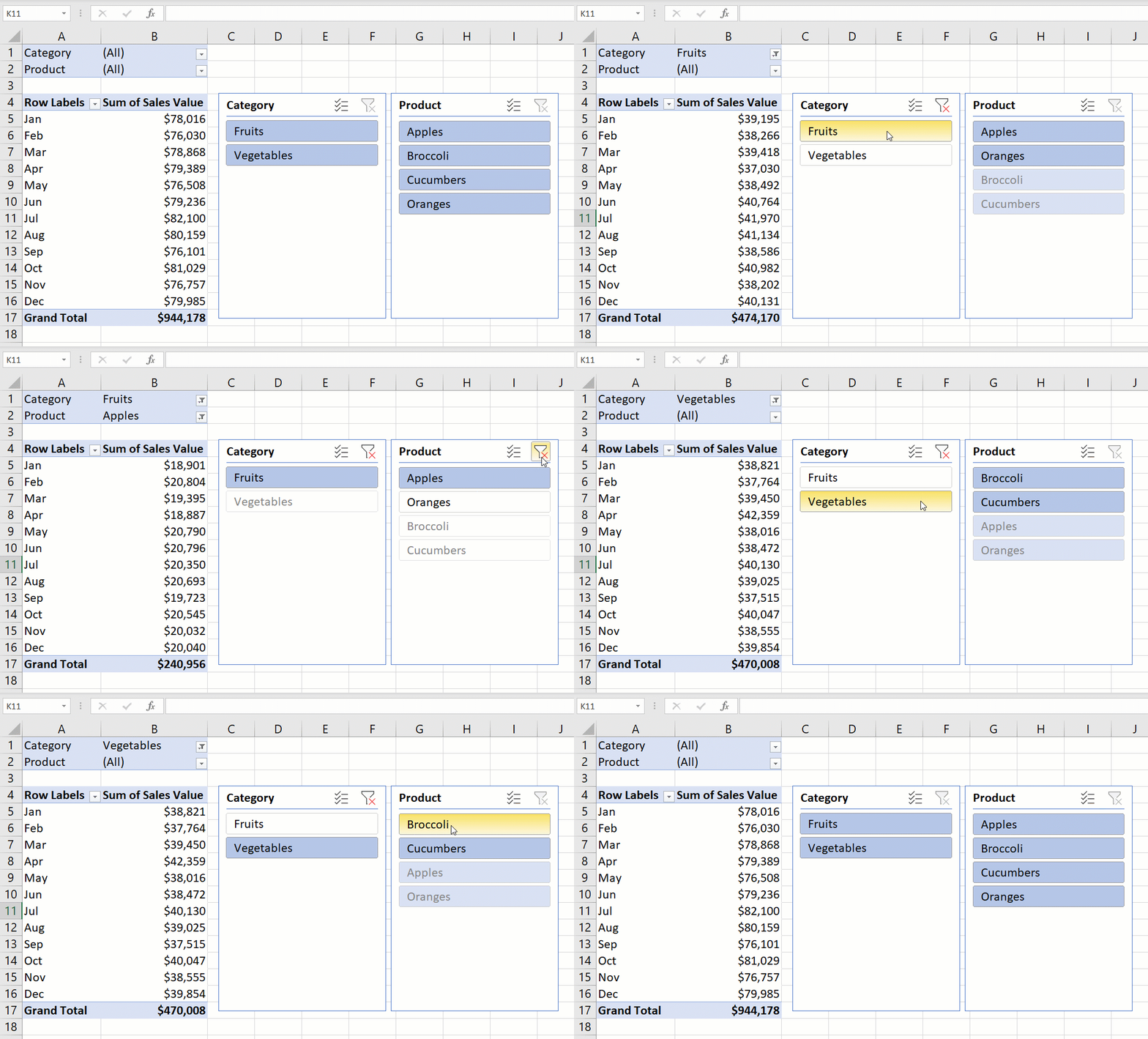
Now watch the power of slicers in the animation below. When you filter the fist Category, Excel does not filter just the pivot table but also filters the available filter options in the Product Category. Now you can choose from the darker colored options that do contain data. Use the top right button in each slicer to clear the filter.

If you want to see this in a video, watch this
