
There are many cases when the data you have in Excel appears to contain dates but when you look closer, the dates are not in a date format. This can be problematic if you need to sort dates, group them by month, year, week or days. So we have to find a way to convert them to a Date format.
The direct text to date conversion
This method may seem very simple and direct. Unfortunately it doesn’t work in most of the difficult cases. However, it is the first method to try so you can see what are you dealing with.
Let’s assume you have some dates written as text in column A. to attempt a direct convert, select the column, right click on it and click on “Format Cells”.
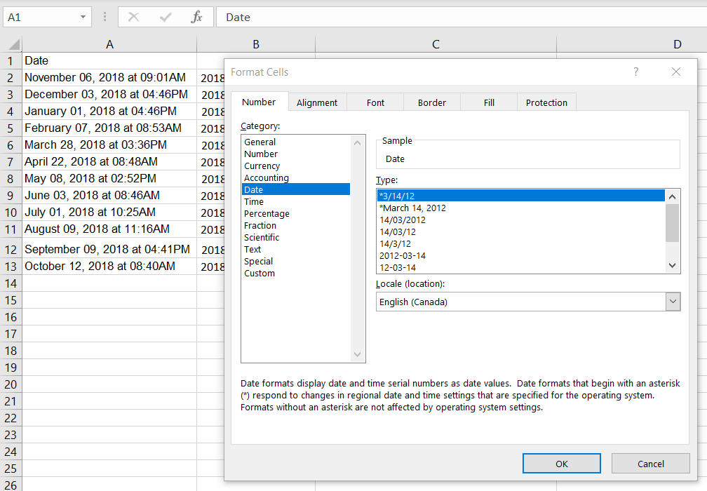
Choose the first date format *3/14/12 (month/day/year) and click OK.
If your date stays the same, then your data is a text and you have to converted following the multi step process below.
Step by Step text to date conversion
The process to convert the text
November 06, 2018 at 09:01AM
into a date
11/06/2018 9:01:00 AM
can be very different depending on the text format. However, the process steps have to follow the two major methods
- Break down all the Date and Time elements (Month, Day, Year, Hour, Minute, Second)
- Build back the Date and Time using the elements.
Let’s get started
Step 1. Break it down
Let’s imagine that date string like it is, a string of characters

To get the month, you have to find a delimiter after the month (space in this case) and take the month name out of the string
- Find the space: B2 = FIND(” “, A2,1) – result is 9, position of the space
- Extract the month: C2 = LEFT(A2,B2-1) – result is November, all characters on the left up to 9-1 (first 8 characters)
- Convert the month to a number: D2 = =MONTH(DATEVALUE(C2&” 1″)) – result will be 11, this is taking out the month out of a string like “November 1”
To get the day, we will go to the right of the delimiter and get the two characters for 06
- Find the Day: =MID(A2,B2+1,2) – result will be 06
To get the year, we’ll look for the next delimiter closer to the year, in this case the comma symbol
- Find the , : F2 = FIND(“,”,A2,1), result will be 12
- Extract the Year: G2 = MID(A2,F2+2,4) – we find the 4 characters for the year 2 spaces to the right so we have to add a 2
To get the hour, we move to the next delimiter “at”
- Find the “at” :H2 = =FIND(“at”,A2,1), result is 19
- Extract the hour: I2 = MID(A2,H2+3,2), we have to move 3 characters to the right from the position of at to find the hour 09
- Extract the minute: J2 = MID(A2,H2+6,2), we move 3 more characters to find the minute
- Find if the hour is AM or PM: K2 = RIGHT(A2,2), find the last two characters on the right
- Turn the hour into a 25 hour format: L2=IF(K2=”AM”,I2+0,I2+12), this will make 9AM into 9 and 9PM into 21
Step 2. Build the Date and Time
Once we broke this string down and we have a day, month and year as well as an hour, minute and second (second will be 00 in this case since we don’t have the information), we can start building back up the Date and the Time
- M2=DATE(G2,D2,E2) – this builds the date
- N2=TIME(L2,J2,0) – this builds the time
- O2 = M2 +N2 – this builds the date/time field
if you want to group all these formulas together, for this case it would look like this:
=DATE(MID(A2,FIND(“,”,A2,1)+2,4),MONTH(DATEVALUE(LEFT(A2,FIND(” “,A2,1)-1)&” 1″)),MID(A2,FIND(” “,A2,1)+1,2)) + TIME(IF(RIGHT(A2,2)=”AM”,MID(A2,FIND(“at”,A2,1)+3,2)+0,MID(A2,FIND(“at”,A2,1)+3,2)+12),MID(A2,FIND(“at”,A2,1)+6,2),0)
Conclusion
The formula above only applies to the string format in this example.
It is important to understand the process of breaking things down and building back up into a date and time field.
If you have a different string format or if you have a challenge, leave a comment and I’ll help you with tips on how to convert various text fields into date