Cell
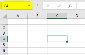
In Excel, one grid box is called a cell. A cell is named as the intersection of the column and row. In the example below, the Cell is named C4 because it is at the intersection of row 4 and column C. You can see the name of the cell that you currently have selected in the name field (highlighted in yellow)
Range
A Range is a collection of two or more cells. If you select a cell and then with the left mouse button pressed, drag the mouse down and right, you would select a range of cell. In the example below I selected 4 cells across 2 rows and 2 columns
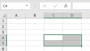
Notice that even though a range of 4 cells is selected, the name still shows only the top left most cell C4. In this case, the Range is not named.
Naming your Range
The selected Range can be named. There are a few reasons for naming a range. One is to be able to quick select it and another reason is so that you can refer the range by name is formulas if you are writing code in VBA later.
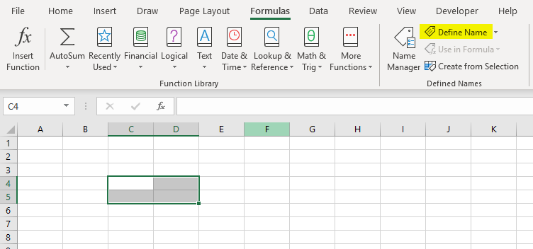
To name a range, select the Range of cell you want to name and go to the Formulas Tab on the Ribbon and in the Defined Names, click on the Define Name button
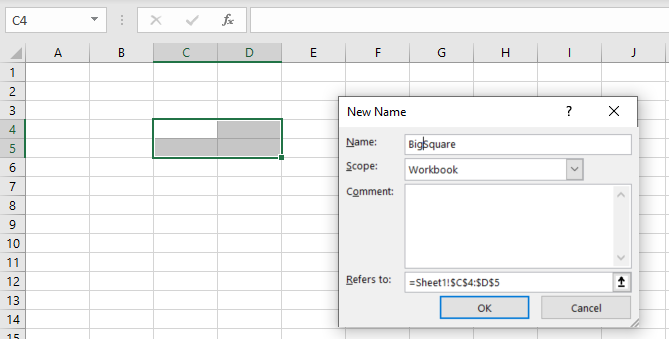
That will open up a dialog box and will invite you to set a name for your Range that you selected. Notice that the Range is already pre-defined IF you had it selected before you clicked on Define Name
Let’s name this Range “BigSquare” and click OK. No spaces or special characters are allowed.
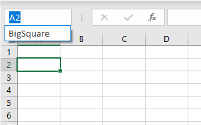
Once you Name a Range, you’ll notice that it is available in the drop down of the Name field
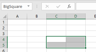
If you select the name BigSquare from the list of names, the Range you wanted is now selected.
Why is this useful?
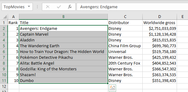
This can be useful if you have a large data set and you want to quickly refer to a range of cells in that data set. Instead of dragging and selecting all the names of the movies in this example data, I just select the Name “TopMovies” and all my movies are now selected. I can now format the entire range, copy it and perform other actions on it.
Fill a Range
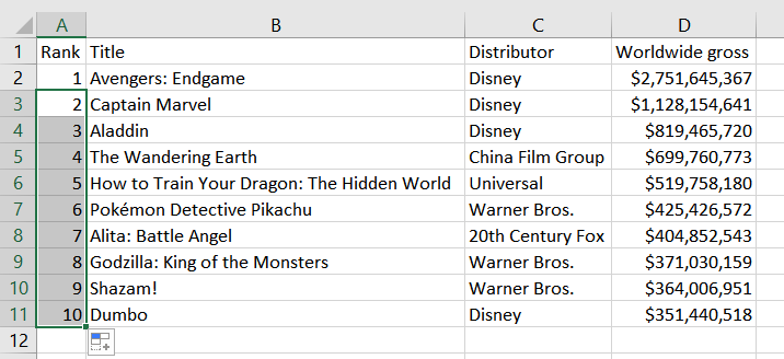
A range of a large data set can be quite large. Let’s suppose we have our list of movies with their worldwide gross revenue and we want to add a rank
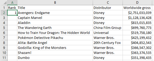
We could create a column called Rank and type in each row a number from 1 to 10
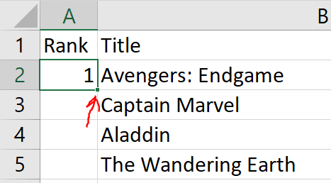
Or we could just type the first number in the rank (1) and fill the rest of the range. To fill the rest of the range, select the small square in the lower right of our selector and holding the mouse button pressed, drag down to fill the range, release the mouse button when done
Well, that didn’t work right? We ended up with all movies ranked as number 1. Disney won’t be pleased.
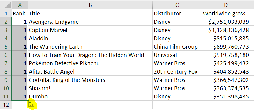
but notice at the bottom of our range there is a small icon. If you hover over that you will notice that this is called Auto Fill Options
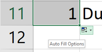
Click on the button and you’ll be presented with the options for your range fill
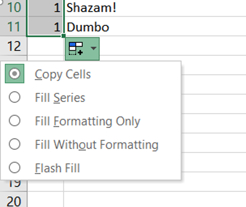
As you can see, the first and the default option is copy cell. You can also Fill Series if you want to create a series from 1 to the last cell. You can also choose to fill with or without formatting and to do a Flash Fill
Choose the Fill Series option to fill the Rank Series with all the ranks from 1 to 10